Weekly Coding Challenge

Every week, we pick a real-life project to build your portfolio and get ready for a job. All projects are built with ChatGPT as co-pilot!

Start the Challenge

Podcast: Code Sets You Free

A tech-culture podcast where you learn to fight the enemies that blocks your way to become a successful professional in tech.

Listen the podcast

Python

Machine Learning

Pandas

Linear Algebra

Edit on Github

Open in Colab

Plotting Functions With Python

Plot functions with Python¶

Ploting data in python is very similar to the process you do in linear algebra: Given a sample of X values you use a function to obtain the Y values an plot the intersection of the X and Y coordinates in the carthesian plane.

In python we use:

The numpy package for obtaining the X and Y values.
The pyplot module of the matplotlib library for ploting and drawing the function.

In [3]:

# import the python module to plot
import matplotlib.pyplot as plt
import numpy as np

If you don't have real data to plot, you can use numpy to generate some sample values, for example:

Here numpy will generate a list of equally distant values from -3 to +3.

In [5]:

x_axis = np.linspace(-3,3)
x_axis

Out[5]:

array([-3.        , -2.87755102, -2.75510204, -2.63265306, -2.51020408,
       -2.3877551 , -2.26530612, -2.14285714, -2.02040816, -1.89795918,
       -1.7755102 , -1.65306122, -1.53061224, -1.40816327, -1.28571429,
       -1.16326531, -1.04081633, -0.91836735, -0.79591837, -0.67346939,
       -0.55102041, -0.42857143, -0.30612245, -0.18367347, -0.06122449,
        0.06122449,  0.18367347,  0.30612245,  0.42857143,  0.55102041,
        0.67346939,  0.79591837,  0.91836735,  1.04081633,  1.16326531,
        1.28571429,  1.40816327,  1.53061224,  1.65306122,  1.7755102 ,
        1.89795918,  2.02040816,  2.14285714,  2.26530612,  2.3877551 ,
        2.51020408,  2.63265306,  2.75510204,  2.87755102,  3.        ])

We can use these values as "seed" or x parameters to obtain the Y values using any linear algebra function. This is an example using the square function.

In [6]:

x_axis = np.linspace(-3,3)

def square(x): return x**2

y_axis = square(x_axis)

plt.plot(x_axis, y_axis)

Out[6]:

[<matplotlib.lines.Line2D at 0x7f79e4a4b490>]

The Parent functions in linear algebra¶

Data patterns can be described by algebra functions and you can plot and visualize them in charts.

The following are called the "parent functions" in linear algebra and the will usually cover 95% of your data patterns.

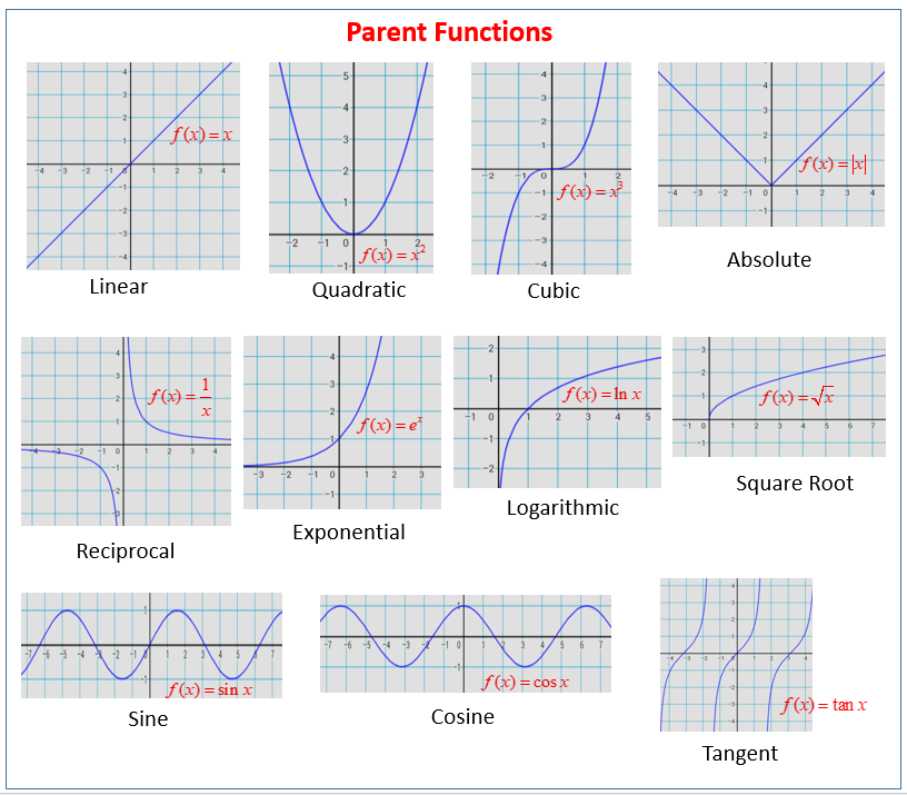
parent functions

Ploting the parent functions¶

Here are some examples of ploting the parent functions in linear algebra, first we import numpy because it contains the functions:

In [2]:

import numpy as np

# start by defining a simple x axis and the Y axis will be given by our parent function
x_axis = np.linspace(-3,3,1000)

Square Function Example¶

In [13]:

def square(x): return x**2
plt.plot(x_axis, square(x_axis))

Out[13]:

[<matplotlib.lines.Line2D at 0x7f97ffe975e0>]

Sen function example¶

In [12]:

def sen_function(x): return np.sin(x)
plt.plot(x_axis, sen_function(x_axis))

Out[12]:

[<matplotlib.lines.Line2D at 0x7f98021a1ea0>]

Exponential Function¶

In [4]:

def explonential(x): return 100*(np.power(2, x))

plt.plot(x_axis, explonential(x_axis))

Out[4]:

[<matplotlib.lines.Line2D at 0x7f8eefdab520>]

Logarithmic Function¶

In [6]:

def logarithmic(x): return np.log10(x)

plt.plot(x_axis, logarithmic(x_axis))

/tmp/ipykernel_2148/3025676228.py:1: RuntimeWarning: invalid value encountered in log10
  def logarithmic(x): return np.log10(x)

Out[6]:

[<matplotlib.lines.Line2D at 0x7f8eedb2feb0>]