Decision Trees

A decision tree is a model widely used in Machine Learning to solve both regression and classification problems. It is a graphical model that mimics human decision making, i.e. it is based on a series of questions to reach a conclusion.

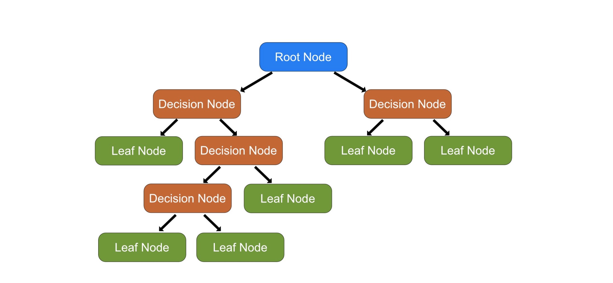
The main idea behind decision trees is to divide data into smaller and smaller groups (called nodes) based on different criteria until a final result or decision is reached. These criteria are selected in such a way that the elements of each node are as similar as possible to each other.

Structure

The structure of a decision tree resembles that of an inverted tree. It starts with a node called root node that contains all the data. This node is split into two or more child nodes based on some criterion. These are the decision nodes. This process is repeated for each child node, creating what are called branches, until a node is reached that is no longer split. These final nodes are called leaf nodes and represent the final decision or prediction of the tree.

An important aspect of decision trees is that they are very interpretable models. You can visualize the entire tree and follow the decisions it makes, which is not possible in many other types of models. However, they can be prone to overfitting, especially if the tree is allowed to grow too large.

Derivation example

Let's imagine we are building a decision tree to decide whether we should play soccer based on weather conditions. We have the following data (in spanish):

Clima	Viento	¿Jugar al fútbol?
Soleado	Fuerte	No
Lluvioso	Débil	Sí
Soleado	Débil	Sí
Lluvioso	Fuerte	No

We start with a single node containing all the data. We need to decide what our first splitting criterion will be, i.e., which of the two features (Clima or Viento) we should use to split the data. This criterion is usually decided based on the purity of the resulting nodes. For a classification problem, a node is pure if all its data belong to the same class. In a regression problem, a node is pure if all the data of that node have the same value for the target variable.

The purpose of splits in a decision tree is to increase the purity of the child nodes. For example, if you have a node that contains spam and non-spam email data, you could split it based on whether the email contains the word "win". This could increase the purity if it turns out that most of the emails that contain the word "win" are spam and most of the emails that do not contain the word "win" are non-spam.

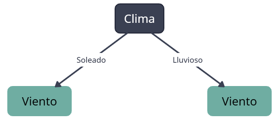
In this case, for simplicity, suppose we decide to divide by Clima first. Then, we split the data into two child nodes: one for sunny days and one for rainy days:

Now we have two child nodes, each with a part of the data:

• In the "Soleado" (sunny) node, we have the following data:

Clima	Viento	¿Jugar al fútbol?
Soleado	Fuerte	No
Soleado	Débil	Sí

• In the "Lluvioso" (rainy) node, we have the following data:

Clima	Viento	¿Jugar al fútbol?
Lluvioso	Débil	Sí
Lluvioso	Fuerte	No

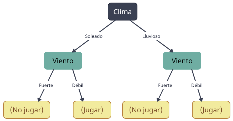
Each of these child nodes is divided again, this time according to wind speed:

Now, each of the child nodes (which are now leaf nodes, since they will not be split anymore because they are pure) represents a final decision based on the weather conditions. For example, if the weather is sunny and the wind is weak, the decision is to play soccer.

Model hyperparameterization

We can easily build a decision tree in Python using the scikit-learn library and the DecisionTreeClassifier and DecisionTreeRegressor functions. Some of its most important hyperparameters and the first ones we should focus on are:

• max_depth: The maximum depth of the tree. This limits how many splits it can have, which is useful to prevent overfitting. If this value is None, then nodes are expanded until leaves are pure or until all leaves contain fewer samples than min_samples_split.
• min_samples_split: The minimum number of samples needed to split a node. If a node has less samples than min_samples_split, then it will not be split, even if it is not pure. Helps prevent overfitting.
• min_samples_leaf: The minimum number of samples that must be in a leaf node. A node will split if doing so creates at least min_samples_leaf samples in each of the children. This also helps to prevent overfitting.
• max_features: The maximum number of features to consider when looking for the best split. If max_features is None, then all features will be considered. Reducing this number may make the model simpler and faster to train, but may also cause it to miss some important relationships.
• Criterion: The function to measure the quality of a split. Depending on the nature of the tree (sort or return), the options vary. This hyperparameter is in charge of choosing which variable to branch.

Another very important hyperparameter is the random_state, which controls the random generation seed. This attribute is crucial to ensure replicability.