Unsupervised learning

Unsupervised learning

Unsupervised learning is a branch of Machine Learning in which hidden patterns and structures in the data are explored and discovered without the guidance of a target variable or prior labels. Unlike supervised learning, where input examples and their corresponding desired outputs are provided to train the model, in unsupervised learning, the algorithm is confronted with an unlabeled data set and seeks to find interesting patterns or group the data into categories without specific guidance.

The main objective of unsupervised learning is to explore the inherent structure of the data and extract valuable information without the model having prior knowledge of the categories or relationships between variables.

There are two main types of unsupervised learning techniques:

1. Clustering: Consists of dividing the data set into groups (clusters) based on similarities or patterns in the data. Clustering algorithms attempt to group similar observations into the same cluster and separate different samples into different clusters.
2. Dimensionality reduction: The objective is to reduce the number of features or variables in the data set without losing important information. These techniques allow the data to be represented in a lower dimensional space, facilitating the visualization and understanding of the data structure.

Unsupervised learning has a wide variety of applications, such as customer segmentation in marketing, data anomaly detection, image compression, document clustering into topics, among others. It is a powerful tool for exploring and understanding the intrinsic structure of data without the need for known labels or answers.

Clustering

Clustering is an unsupervised learning technique used to divide a dataset into groups based on similarities between observations. The objective is to group similar items into the same cluster and to separate different observations into distinct clusters, without having prior information about the categories to which they belong.

There are several clustering algorithms, but the most common are:

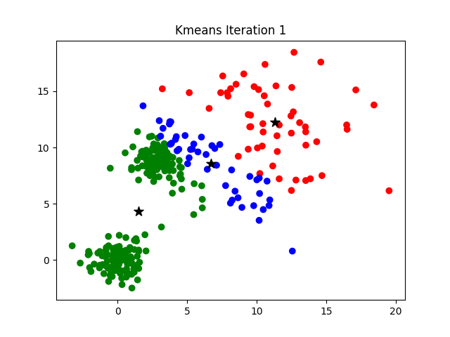
• K-Means: This is one of the most popular clustering algorithms. It starts by defining random K centroids (point representing the geometric center of a cluster), then assigns each data point to the nearest centroid and recalculates the centroids as the average of the assigned points. Repeat this process until the centroids converge.
• Hierarchical Clustering: It starts by considering each data point as its own cluster and gradually merges the nearest clusters into one. This forms a hierarchy that can be represented in a dendogram.
• DBSCAN (Density-Based Spatial Clustering of Applications with Noise): Clusters data points that are close to each other and have enough neighbors in their neighborhood. It allows finding clusters of irregular shapes and sizes and also detecting outlier points.

K-Means

The K-Means algorithm is a clustering technique that aims to divide a dataset into K clusters (defined as input parameter), so that points within each cluster are similar to each other and different from points in other clusters.

It is an iterative process composed of several steps:

1. Initialization. The process begins by defining K random points in the data set as initial centroids. The centroids are representative points that will serve as the initial centers of each cluster.
2. Assignment of points to clusters. Each point in the data set is assigned to the cluster whose centroid is the closest. This is done by calculating the distance between each point and the centroids, and assigning the point to the cluster whose centroid has the smallest distance. The distances used and available are the ones we studied in the KNN model module and can be found here.
3. Centroid update. Once all points are assigned to their corresponding clusters, the centroids are updated by recalculating their position as the average of all points assigned to that cluster. This step relocates the centroids to the geometric center of each cluster.
4. Iteration. Steps 2 and 3 are repeated until the centroids no longer change significantly and the points are stable in their clusters. That is, the algorithm continues to assign and update points until convergence is reached.
5. Result. Once the algorithm has converged, the points in the data set are grouped into K clusters or groups, and each cluster is represented by its centroid. The groups obtained represent sets of similar points.

The challenge of finding the optimal K can be addressed by hyperparameter optimization or by more analytical procedures such as the elbow method, more information about which can be found here.

This algorithm is fast and effective for data clustering, but it is highly dependent on the initial centroid distribution and does not always find the best overall solution. Therefore, it is sometimes run several times with different initializations to avoid obtaining suboptimal solutions.

Implementation

The implementation of this type of model is very simple, and is carried out with the scikit-learn library. For this purpose, we will generate a sample example using this library as well:

1import numpy as np
2from sklearn.cluster import KMeans
3from sklearn.datasets import make_blobs
4
5# Generate a sample dataset
6X, _ = make_blobs(n_samples = 300, centers = 3, random_state = 42)
7
8# Training the model
9model = KMeans(n_clusters = 3, random_state = 42)
10model.fit(X)
11
12# Making predictions with new data
13new_data = np.array([[2, 3], [0, 4], [3, 1]])
14predictions = model.predict(new_data)

In this example code we generate 2 clusters (hyperparameter n_clusters) and set the seed since it is a model with a random initialization component.

Once we have trained the model we can get the labels of which cluster is associated to each point with the labels_ attribute of the model (model.labels_). We can also obtain the coordinates of the centroids of each cluster with the cluster_centers_ attribute of the model (model.cluster_centers_).

Hierarchical Clustering

Hierarchical clustering is a clustering technique that organizes data into a hierarchy of clusters, where smaller clusters are gradually combined to form larger clusters. The end result is a dendrogram, which is a graphical representation of the cluster hierarchy.

It is an iterative process composed of several steps:

1. Initialization. Each data point is initially considered as its own cluster.
2. Similarity calculation. The similarity or distance between all pairs of data points is calculated. The distances used and available are the ones we studied in the KNN model module and can be found here.
3. Cluster union. The two closest clusters are combined to form a new larger one. The distance between two clusters can be calculated in many ways.
4. Similarity matrix update. The similarity matrix is updated to reflect the distance between the new clusters and the remaining clusters.
5. Iteration. Steps 3 and 4 are repeated until all data points are in a single cluster or until a specific number of desired clusters (input hyperparameter) is reached.
6. Dendogram. The result of hierarchical clustering is displayed in a dendogram, which is a tree diagram showing the hierarchy of the groups. The data points are located at the leaves of the tree, and larger clusters are formed by combining smaller clusters along the branches of the tree.

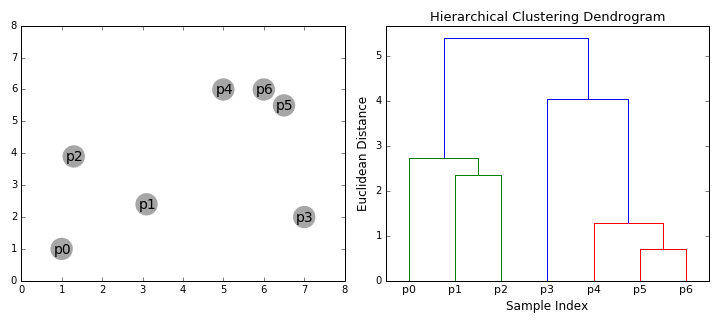
The dendrogram allows visualizing the hierarchical structure of the clusters and the distance between them. The horizontal cuts in the dendrogram determine the number of clusters obtained by cutting the tree at a certain height.

Hierarchical clustering is useful when the optimal number of clusters is not known in advance or when it is desired to explore the hierarchical structure of the data. However, it can be computationally expensive on large data sets due to the need to calculate all distances between data points.

Implementation

The implementation of this type of model is very simple, and is carried out with the scipy library. To do so, we will generate a sample example using the scikit-learn library:

1import numpy as np
2from scipy.cluster.hierarchy import dendrogram, linkage
3from sklearn.datasets import make_blobs
4
5# Generate a sample dataset
6X, _ = make_blobs(n_samples = 100, centers = 3, random_state = 42)
7
8# Calculate the similarity matrix between clusters
9Z = linkage(X, method = "complete")
10
11# Display the dendrogram
12plt.figure(figsize = (10, 6))
13
14dendrogram(Z)
15
16plt.title("Dendrograma")
17plt.xlabel("Índices de datos")
18plt.ylabel("Distancia")
19plt.show()

We could also use the scikit-learn library to implement this model, using the AgglomerativeClustering function, but nowadays the scipy version is more widely used because it is more intuitive and easier to use.

Dimensionality reduction

Dimensionality reduction is a technique used to reduce the number of features or variables in a data set. The main objective of this model is to simplify the representation of the data while maintaining as much relevant information as possible.

In many data sets, especially those with many features, there may be redundancy or correlation between variables, which can make analysis and visualization difficult. Dimensionality reduction addresses this problem by transforming the original data into a lower dimensional space, where the new variables (called principal components or latent features) represent a combination of the original variables.

There are two main approaches to dimensionality reduction:

• Principal Component Analysis (PCA): Is a linear technique that finds the directions of maximum variance in the data and projects the original data into a lower dimensional space defined by the principal components. The objective is to retain most of the variance in the data while reducing the dimensionality of the data.
• Singular Value Decomposition (SVD): A mathematical technique used to factorize a data matrix into three components: which are then used to reduce the dimensionality.

There are many reasons why we would want to use this type of model to simplify the data. We can highlight:

1. Data simplification and visualization: In data sets with many features, dimensionality reduction makes it possible to simplify the representation of the data and to visualize them in lower dimensional spaces. This facilitates the interpretation and understanding of the data.
2. Noise reduction: By reducing dimensionality, redundant or noisy information can be removed, which can improve data quality and the performance of machine learning models.
3. Computational efficiency: Feature-rich datasets may require increased computational and memory capacity. Dimensionality reduction can help reduce this complexity, resulting in faster training and prediction times.
4. Regularization: In some cases, dimensionality reduction acts as a form of regularization, avoiding overfitting by reducing the complexity of the model.
5. Feature exploration and selection: Dimensionality reduction can help identify the most important or relevant features of a dataset, which can be useful in the EDA feature engineering process.
6. Data preprocessing: Dimensionality reduction can be used as a preprocessing step to improve data quality before applying other machine learning algorithms.

PCA

The PCA is a dimensionality reduction technique that seeks to transform an original data set with multiple features (dimensions) into a new data set with fewer features, but preserving most of the important information.

Imagine that we have a dataset with many characteristics, such as height, weight, age, income and education level of different people. Each person represents a point in a high-dimensional space, where each feature is a dimension. PCA allows us to find new directions or axes in this high-dimensional space, known as principal components. These directions represent the linear combinations of the original characteristics that explain most of the variability in the data. The first principal component captures the largest possible variability in the data set, the second principal component captures the next largest variability, and so on.

When using PCA, we can choose how many principal components we wish to keep. If we choose to keep only a few of them, we will reduce the number of features and thus the dimensionality of the data set. This can be especially useful when there are many features and we want to simplify the interpretation and analysis of the data.

Implementation

The implementation of this type of algorithm is very simple, and is carried out with the scikit-learn library. We will use a dataset that we have been using regularly in the course; the Iris set:

1from sklearn.datasets import load_iris
2from sklearn.decomposition import PCA
3
4# Load the Iris dataset
5iris = load_iris()
6X = iris.data
7y = iris.target
8
9# Create a PCA object and fit it to the data
10pca = PCA(n_components = 2)
11X_pca = pca.fit_transform(X)

The n_components hyperparameter allows us to select how many dimensions we want the resulting dataset to have. In the example above, there are 4 dimensions: petal_length, petal_width, sepal_length and sepal_width. We then transform the space into a two-dimensional one, with only two features.